The Compound Interest Theorem in Excel Formulas

Compound interest is a powerful concept in finance that allows investments to grow exponentially over time. Unlike simple interest, where interest is calculated only on the principal amount, compound interest takes into account both the principal and the accumulated interest from previous periods.

In simple terms, compound interest allows money to grow exponentially. The basic idea is that as interest accumulates, it becomes part of the principal for the subsequent periods, leading to a compounding effect. This compounding effect results in the interest being calculated not just on the original amount but also on the interest that has already been added.

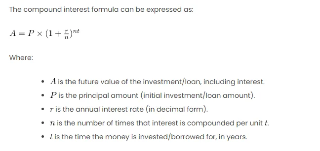
The Compound Interest Theorem is expressed in a formula where the future value ( $A$ ) of an investment or loan is determined by the principal amount ( $P$ ), the annual interest rate ( $r$ ), the number of compounding periods per year ( $n$ ), and the duration of the investment or loan ( $t$ ). This formula enables individuals and businesses to project the growth of their investments or the cost of their loans over time.

The compound interest formula can be expressed as:

$A = P \times (1 + \frac{r}{n})^{nt}$

Where:

$A$ is the future value of the investment/loan, including interest.
$P$ is the principal amount (initial investment/loan amount).
$r$ is the annual interest rate (in decimal form).
$n$ is the number of times that interest is compounded per unit $t$ .
$t$ is the time the money is invested/borrowed for, in years.

Excel Formulas for Compound Interest

In Excel, you can use the following formula to calculate compound interest:

= P * (1 + r/n)^(n*t)

Now, let’s break down the steps to use this formula in Excel:

Input Parameters: Enter the principal amount ( $P$ ), annual interest rate ( $r$ ), the number of times interest is compounded per year ( $n$ ), and the time the money is invested/borrowed for ( $t$ ) in separate cells.
Excel Formula: In a cell, enter the compound interest formula using the cell references for the input parameters.
Calculate Compound Interest: After entering the formula, Excel will automatically calculate the compound interest based on the provided parameters.

Explanation with Scenario

Let’s consider a scenario to illustrate the compound interest formula:

Principal ( $P$ ): $10,000
Annual Interest Rate ( $r$ ): 5%
Compounding Frequency ( $n$ ): 4 times per year
Time ( $t$ ): 3 years

Now, using the formula, we can calculate the compound interest in Excel:

=P * (1 + r/n)^(n*t)

The result will be the future value ( $A$ ) of the investment after 3 years.

Excel Table for Visualization

Consider the following Excel table for a clear visualization:

Parameter	Value
Principal ( $P$ )	$10,000
Annual Interest Rate ( $r$ )	5%
Compounding Frequency ( $n$ )	4 times per year
Time ( $t$ )	3 years
Compound Interest Formula	`=A2 * (1 + B2/C2)^(C2*D2)`
Result (Future Value)	Excel Formula Result

Calculation and Result

Plugging in the values into the formula:

=10000 * (1 + 0.05/4)^(4*3)

The result is approximately $11,576.53. Therefore, the future value of the investment after 3 years with compound interest is $11,576.53.

Other Approaches

Excel Functions: Excel also provides functions for compound interest, such as FV (Future Value) and RATE (Interest Rate). These can be used as alternatives.
Data Tables: Excel’s Data Table feature can help you create multiple scenarios by changing one or more input parameters, allowing you to analyze how different values affect the compound interest.